How to treat Overfitting in Convolutional Neural Networks
Jul 11, 2020

In this tutorial you would learn some methods that can be used to improve a model’s accuracy using deep learning neural networks. This can be achieved in a few lines of code using Tensorflow by just importing required libraries. If you haven’t already, you can build a Tensorflow Image Classification model following the guide in the last post How to Build an Image Classification API in Tensorflow. This is an overview of what we would be touching on in this tutorial:
Overview
- Improving Model’s Accuracy
- Dropouts: Understanding how it reduces Overfitting
- Batch Normalization
- Buiding a Cifar10 Model with 85% Accuracy
Previous: How to Build an Image Classification API in Tensorflow
Next: Building an Image Classification API with TFX and GCP
Improving Model's Accuracy with Convolutional Neural Networks
In the last article we built a simple classifier model in Tensorflow. I achieved 75% accuracy after evaluating the test set which consists of 10000 Images which was not used in training. This gives us a view of how our model would perform in a real world scenario. Of-course, we aren’t going to use this model for any big projects anytime soon, but by practising on it gives us understanding that can be applied to bigger projects.
Not all model’s after training can be significantly improved by applying this methods. It could be that the achitecture used at first didn’t train the model in the right way. In this case, you would need to change the layers used before getting any significant improvements. A very good way of knowing if a model can be improved is by plotting learning curves. This can be done in tensorflow in just a few lines of code.
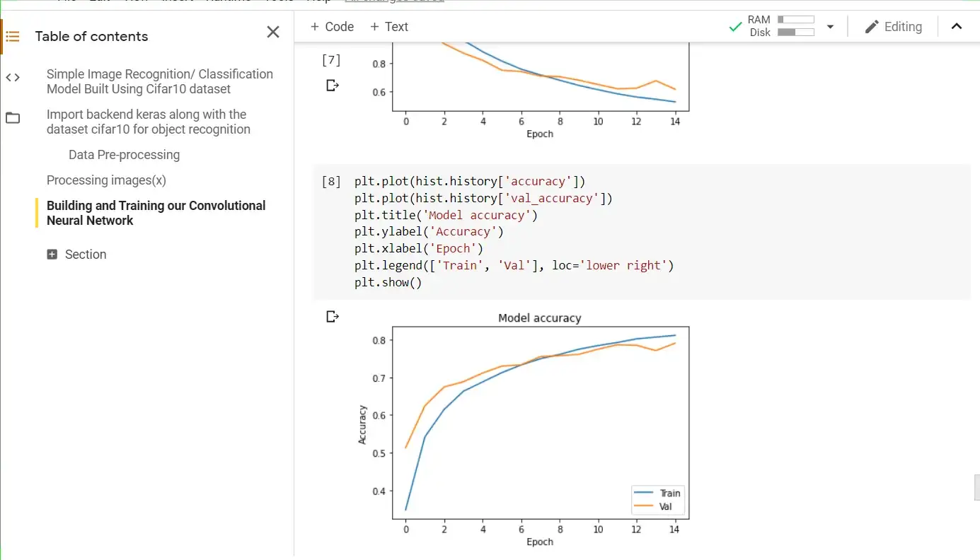 As seen in the image above, around epochs 14, the validation set curve (orange) can be seen to have a strong dip. This tells us that if we increase the number of epochs or add regularization techniques like Dropouts and BatchNormalization, we can achieve better accuracy
In this tutorial, we would look at some established methods of reducing overfitting and slowing-down convergence in our model which in turn gives us better accuracy. Let’s look at them now.
Dropouts
Dropout is a technique for addressing overfitting. The main idea here is for our neural network to randomly drop units during training. The reduction inparameters in each step of training has effect of regularization. Dropout has shown improvements in the performance of neural networks on supervised learning tasks in vision, speech recognition, document classification and computational biology, obtaining state-of-the-art results on many benchmark data sets.
BatchNormalization
BatchNormalization normalizes the activation of the previous layer at each batch, i.e. applies a transformation that maintains the mean activation close to 0 and the activation standard deviation close to 1. It addresses the problem of internal covariate shift. It also acts as a regularizer, in some cases eliminating the need for Dropout. Batch Normalization achieves the same accuracy with fewer training steps thus speeding up the training process. This definition is cited from appliedmachinelearning.blog
Now that we understand the technique that would be applied during training to improve accuracy, let’s see how to implement it in code.
Buiding a Cifar10 Model with 85% Accuracy
Below is the code that introduces batch normalization and dropouts to our model’s ConvNet. For the full code including loading the dataset and normalizing it, refer to my github repo here Image Classification with Cifar10 (Full)
from keras.models import Sequential
from keras.optimizers import SGD
from keras.preprocessing.image import ImageDataGenerator
from keras.layers import BatchNormalization
from keras import regularizers
from keras.callbacks import LearningRateScheduler
from keras.layers import Dense, Dropout, Flatten, Conv2D, MaxPooling2D

model = Sequential()
model.add(Conv2D(32, (3, 3), activation='relu', padding='same', input_shape=(32, 32, 3))),
model.add(Conv2D(32, (3, 3), activation='relu', padding='same'))
model.add(MaxPooling2D(2, 2)),
model.add(Dropout(0.2))
model.add(Conv2D(64, (3, 3), activation='relu', padding='same')),
model.add(Conv2D(64, (3, 3), activation='relu', padding='same')),
model.add(MaxPooling2D(2, 2)),
model.add(Dropout(0.2))
model.add(Conv2D(128, (3, 3), activation='relu', padding='same')),
model.add(Conv2D(128, (3, 3), activation='relu', padding='same')),
model.add(MaxPooling2D(2, 2)),
model.add(Dropout(0.2))
model.add(Flatten()),
model.add(Dense(512, activation='relu')),
model.add(Dropout(0.5))
model.add(Dense(10, activation='softmax'))

model.summary()

model.compile(loss='categorical_crossentropy',
              optimizer='adam',
              metrics=['accuracy'])

hist = model.fit(x_train, y_train_one_hot,
          batch_size=64, epochs=25,
           validation_split=0.2, verbose=1)
The output of the above code implementation for Image classification task is shown below:
Here, we trained our model for just 25% accuracy and achieved approx 85% accuracy. This is a significant development from when we only convolution and maxpooling layers to build our model. Training it for more epochs can as well give you more accuracy which you should try out by simply following the guide.