How to Build an Image Classification Model and Web App with Tensorflow

Jun 28, 2020

In this tutorial, you would learn how to build an Image Classification Model using Tensorflow on Google Colab. This tutorial is the first among three set. They go from buiding an Image Classifier to Improving accuracy in your model and finally Serving it for production through an API url Endpoint. To start off, here is the overview of all what we would be touching on.

Overview

• Image Classification In Computer Vision
• Applications of Image Classification in World Industry
• Steps to Build an Image Classification Model
• Building the Model with Tensorflow (Keras)

Next: Improving your Tensorflow Model with Regularization

Finally: Building an Image Classification API with TFX and GCP

Now that you have an idea of the steps taking us through this tutorial, Let’s begin with it.

Introduction

Starting off in Machine Learning and Deep Learning can be Overwhelming, I say this because I’m currently in the process of experiencing the start off altogether. There are so many fields, opinions, doubts that can go through your mind on the process of choosing a path to follow. Sometimes, actually most times, It’s really cool to look at the big guys in the field that exude so much confidence showing that they know what they want. Also, there are lots of resources and articles around promising ways that would become a revelation to newcomers and map out the correct path for them. I just read some of those, and I’m more affected than when I was using my mind at a space to think for myself. My mood becomes let’s say negative. But I can’t be like that for long. I simply told myself I’m gonna learn them all by “doing”. It’s a big deal, perhaps the hardest part but with time it becomes a natural thing for you. That’s the way of life. Long story short, I decided to start implementing projects that I could add to my github, LinkedIn and blog.

This tutorial is mainly for people starting off in “Computer Vision”, those that want to “know” and “do” Computer Vision. What I want you to understand is this: “It’s all in the process. Those little steps sums into the big advancement”.. Well, at least I told myself that. OpenCV can wait, I’m gonna learn all the small steps involved but I’m gonna learn them very fast. I have the ability to, and I hope with the series of upcoming posts, you too can follow along and master the baby steps in Computer Vision(CV). Let’s get into more concrete writings.

Image Classification In Computer Vision

The term Image Classification, a deep learning task refers to a task in CV that involves the process of assigning classes to an entire image or picture. It is sometimes referred to as Image recognition, which is a broader term that refers to various tasks that involves classifying the content of images.

The task of helping computers to see, and make a sense or add meaning to what they see is a very hard task. Mainly because it does not just involve one but a series of steps are involved owning to the fact that real-world data or scenerio is unpredictable. Therefore, this is no longer a common task of pre-programmed rules giving accurate results. For computers to see, at basic level, they have to understand single still images before processing advanced high fps videos of which is our general goal as ML engineers and researchers.

We come now to the problem of helping computers see. In accord, I decided to start of with the simplest problem and I think that should be Image Classification. In this problem

• We take a dataset that consists of a set of items in images and their corresponding labels
• We train a model using the dataset so it can make predictions on new images by correctly assigning them to the right class
• If it sees an image not among the class it was trained on, it would give it the label of the output with the highest probability
• This tells us that if we want a model to recognize a thousand different items accurately, we would train it with a dataset outlining those items and their respective label. But ofcourse, this is not an effecient way of tackling the problem. We have millions of items in the world, not to talk of species of animals..xD

As simple a task as Image Classification is it has some very impressive applications that has been very beneficial to diiferent industries. Let’s look at some Applications:

Applications of Image Classification in World Industry

• In Manufacturing: A system built with a classification model can help speed up production process by efficiently reporting bad/damaged items before they are packaged for distribution. By classifying items as bad or good after being trained with a lot of data in the respect of it’s use-case. The main benefit of this is that, it does this considerably faster than human workers and workforce is also reduced resulting in the decrease in “cost of production”, which in a way can lead to cheaper products.

• In Medical: An image classifiction system trained with a lot of medical X-ray records depicting a patient eith a disease vs one without can be used to accurately diagnose the health condition of new patients. This can significantly reduce the time spent by medical practitioners conducting several tests before giving results, therby giving them more time to focus on other matters.

• In Computer Vision: Image classification is a very important application in CV fields. At a basic level, it makes up the structure of an Object detection system which involves “localizing objects in an image by drawing a bounding box around them while also assigning objects to their correct class”. Image classification is used as the basis of many advanced CV applications, a good example is an autonomous vehicle. Image classification and Object detection is the main components making up the system though at advanced level. A self-driving car has to recognize objects it should not hit like pedestrains and road signs, it also has to localize them to undestand their path. This is a clear example of video/moving object detection.

• In Agriculture: Models built on Image classification has a tremendous impact in the agricultural sector. They can be applied to numerous problems and can give very accurate results that significantly improves the conditions ans returns of farming. A popular example is an app built in Tensorflow that is used to identify early on, cassave crops with high probability of disease infection. This can help farmers increse yield / decrese loss by being aware of the health of their crops in advance.

There are so many other applications of Image classification not mentioned. What I like best about ML models is that they make we humans more productive anywhere which they are applied. And that is why we keep researching ways to make them easier to build, cost effective and being able to be used for more complicated problems.

Now I just gave some applications, another fun applications is integrating them in web and mobile applications for a number of services partaining to businesses. Today , you would build a classification model and use it as the backend of a web app. Now let’s look at the steps to build this model:

In this tutorial, I’m using the Tensorflow ML framework and Keras backend. You dont need to install Tensorflow if you dont have it, we would be writing all the code in Google Colab, you can follow this link to open colab and create a new file … Open Google Colab

Steps to build an Image Classification Model

• Import Keras and load Cifar10 Dataset

• Understanding our Dataset & Image (shape)

• Data Pre-processing

• Image Processing

• Understanding the Stucture of Model

• Building and Training a ConvNet for Image Classification

if you are a total beginner and don’t understand some the terms used Like ConvNet, Image Processing and so on, I recommend taking this course by deeplearning.ai on Tensorflow. Or you can contact we directly giving me and I can recommend some resources that should help you get started.

We want to start by importing Kera which would be what we use to build our model. Cifar10 is a dataset consisting of 10 different items and their corresponding label. We are gonna use this to train a model.

My aim is to build a web application that uses the complete trained model as a back-end through an API endpoint. This web app would perform object recognition on images when a user uploads a given image and it would then using probability, pass as results the most likely class the object in that image belongs to. As expected, this would only work on 10 different classes of images from real-world examples making the user very limited in the amount of images he can classify( not that he doesn’t know the class of that image). In the next tutorial we can try out thsi same problem but on a larger dataset mainly Cifar100 i.e with 100 class of things. Let’s start writing some code!

• Use the following lines below to import keras along with cifar10
• Store the data in the respective arrays to be used for training

After those simple steps are completed, we can use the print function to see the shape of our training images

from keras.datasets import cifar10
(x_train, y_train), (x_test, y_test) = cifar10.load_data()
print('x_train shape:', x_train.shape)
print('y_train shape:', y_train.shape)
print('no_of_x_train:', len(x_train))

Output: 
x_train shape: (50000, 32, 32, 3)
y_train shape: (50000, 1)
no_of_x_train: 50000S

By running that piece of code,, we get the following output above. The shape of x_train printed out is (50000, 32, 32, 3). In simple words, the shape of our array tells us that our x_train consists of:

1. 50000 images (training data)
2. 32 pixels in height (images)
3. 32 pixels in width
4. 3 pixels in depth (RGB values of image)

For our label training data y, we get the shape output as (50000, 1). This tells us we have 50000 label data in our training set with just one value

That is the shape of our training data but keras stacks them in a 4D format, for easier processing when building our model. Now let’s try to see a full example of an image and label to better understand the logic. The code below helps us to that.

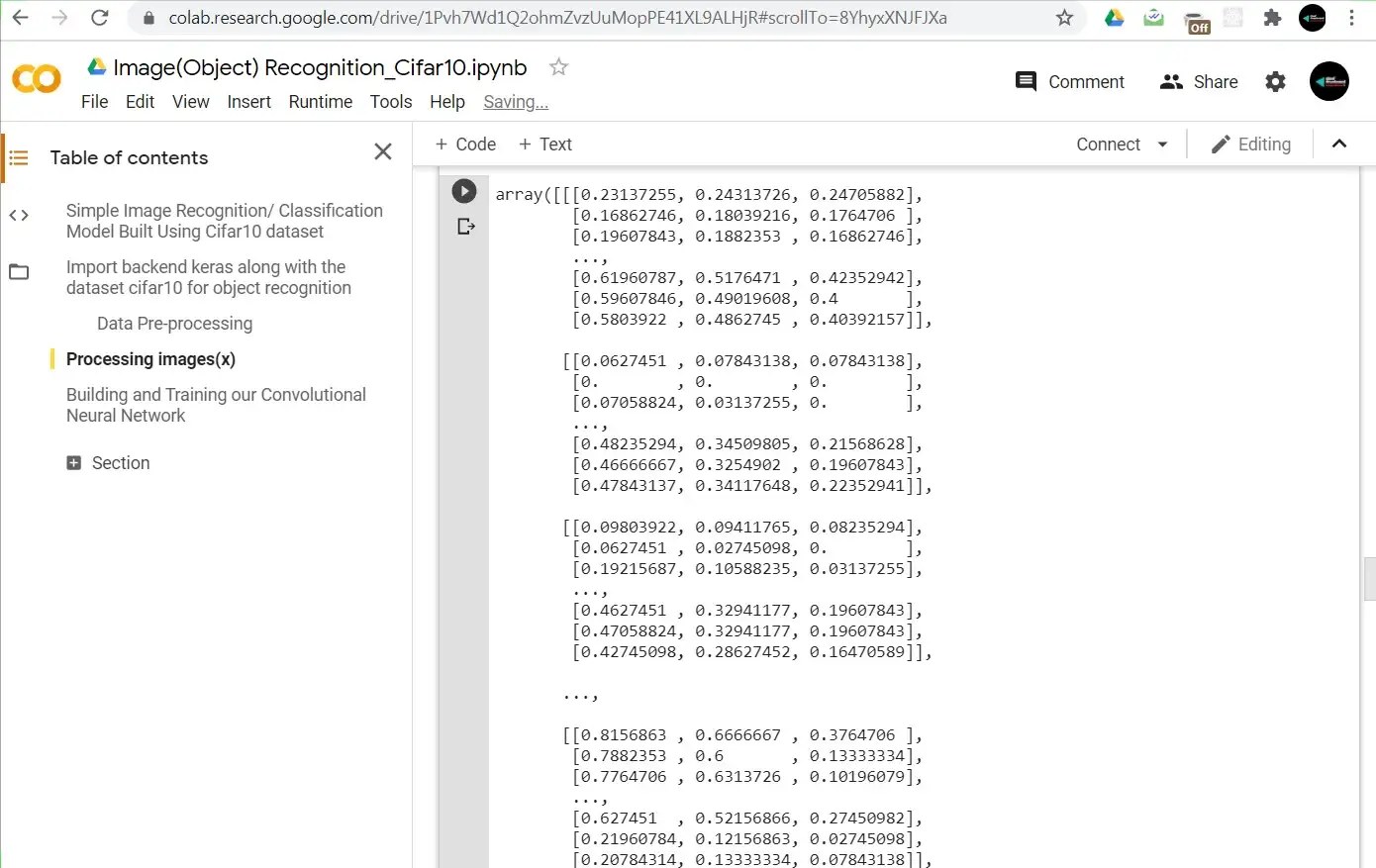
print(x_train[0])

The output looks like the image below:

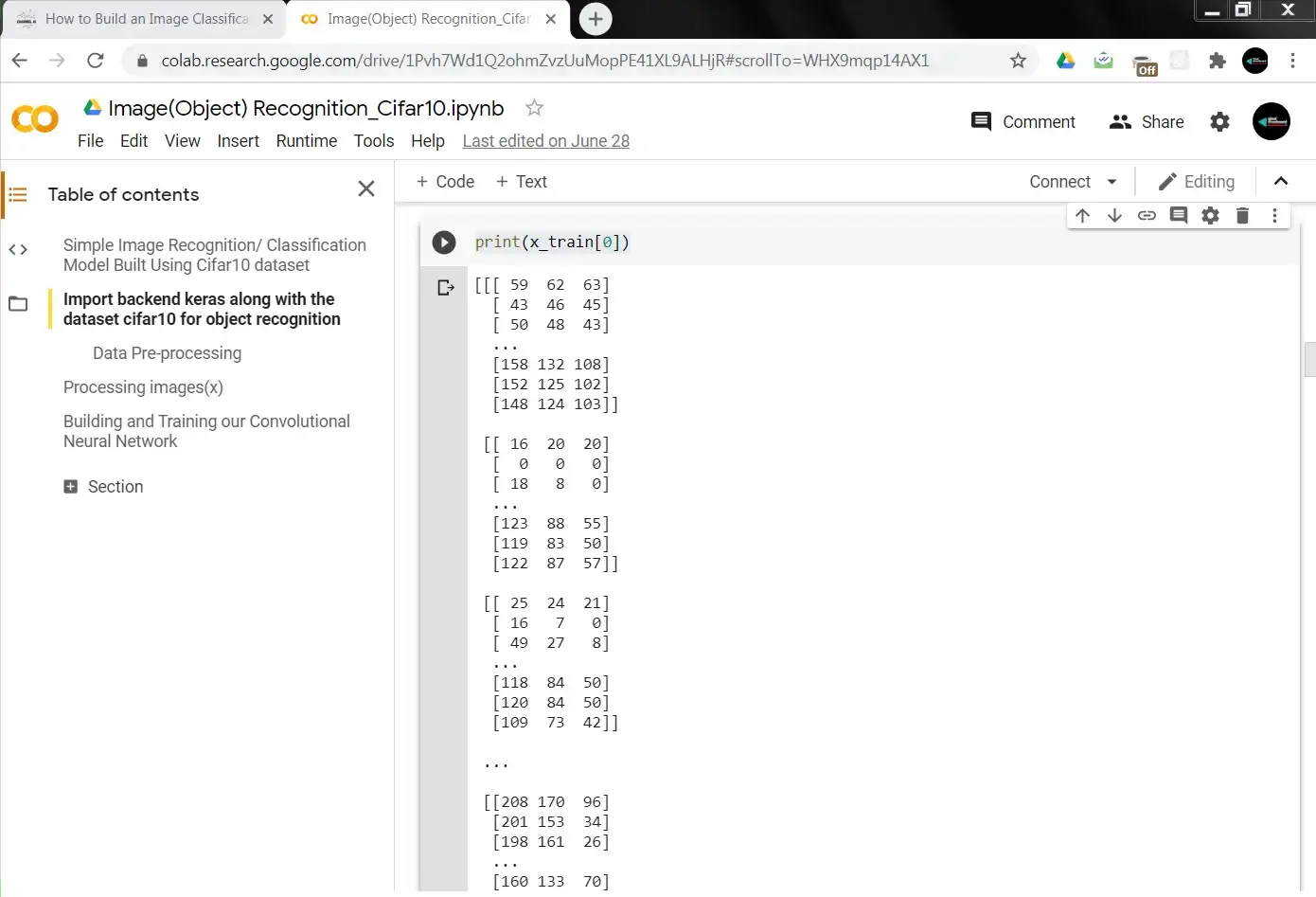
Trying to visualize the image this way doesn’t help us a lot, although that’s how it is interpreted for the computer. The Red, green, and blue values in our 3 byte image are just a bunch of numbers that the computer can use to calculate the intensity of r,g,b at a pixel point. We can use the matplotlib package for a finer, data plot. Let’s import the package in the next lines of code

Note: imshow is a function that maps the numbered pixel values of x_train[0] like we saw previously, into the actual image it represents.We also print out the label, that is, the class this image belongs to of the 10 classes we have. Classes begin from index 0.

import matplotlib.pyplot as plt
img = plt.imshow(x_train[1])

print('The label is:', y_train[1])

Output:
The label is: [9]

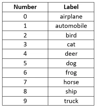
The label showing as nine means that the second image in our training set (following index: 0 is first_img, 1 is second_img ) has a label/class of 9(truck) i.e the very last of the classes. With this we still do not know the class in words representing this image. The below image shows the conversion of numbers to the word class. Change the value of the printed x’s and labels in your colab environment, and visualize the different classes that gets printed out.

Data Pre-processing

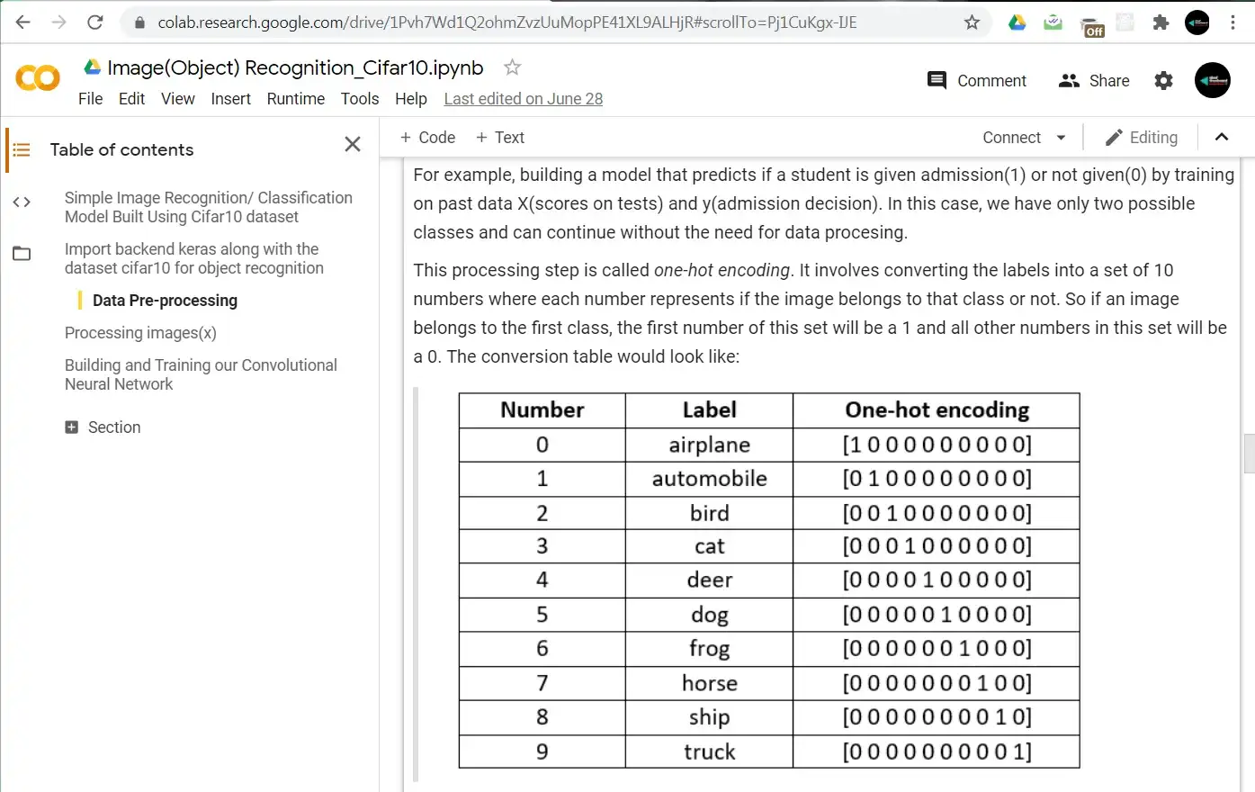
In this step we want to preprocess our data because our labels as class number are not very helpful. We can hot-encode our label so that the model returns 1 for matched class and 0 for the rest unmatched classes(i.e 9,since there would always be one matched class). For a simple binary-logistic predictor, we would not need to perform this pre processing step mainly because our classes are just two. Class 0 and class 1. For example, building a model that predicts if a student is given admission(1) or not given(0) by training on past data X(scores on tests) and y(admission decision). In this case, we have only two possible classes and can continue without the need for data procesing.

We can call our current problem a multi-variant/multi-label logistic problem. Using traditional Machine Learning method of mapping x’s to their labels, we would have to build a classifyer for all our 10 classes and optimize each of them separately,i.e 10 seperate theta parameter. But thankfully, we are using a framework that abstracts much of the work for us.

This processing step is called one-hot encoding. It involves converting the labels into a set of 10 numbers where each number represents if the image belongs to that class or not. So if an image belongs to the first class, the first number of this set will be a 1 and all other numbers in this set will be a 0. The conversion table would look like:

Now here we have been talking about one-hot encoding for a while, let’s write code for it in a few lines:

import keras
y_train_one_hot = keras.utils.to_categorical(y_train, 10)
y_test_one_hot = keras.utils.to_categorical(y_test, 10)

print('The one hot label is:', y_train_one_hot[1])

Output: 
The one hot label is: [0. 0. 0. 0. 0. 0. 0. 0. 0. 1.]

In the above code, the line y_train_one_hot = keras.utils.to_categorical(y_train, 10) means that we want to take the array conatining the number labels of y_train and convert it to one-hot setting y_train_one_hot. The numeber 10 is a required paarmeter, it specifies the number of classes there are.

We printed out the label of our second image(index 1/truck/label 9) and got the one-hot setting as above.

Processing Images(x)

To process our images , what we do is reduce the pixels values between 0 and 1 which would aid in training our neural network. The pixel values of x ranges between 0 - 255, to reduce them we can divide b 255. We first covert the datatype to float32 which is a datatype that can store decimal values. Let’s write code for this.

We process our images before training mainly for our convolutions to easily find features to use for training therby reducing training period

x_train = x_train.astype('float32')
x_test = x_test.astype('float32')

x_train = x_train / 255
x_test = x_test / 255

x_train[0]

When we print our output,, like previously we get a bunch of numbers except that this time around they all fall in the range of 0 and 1. The process of reducing our image pixels in this way is called Normalization

This processing step makes our neural network to train faster and achieve better accuracy. Note: This processing is also carried out on the test set since when evaluating we want the same range of values as those used when training.

Understanding the Stucture of Model

We finally arrive at the most productive step, to train our model. This step just involves setting up a structure or architecture we want our model to have. We would add layers to our model in these sequence:

1. Add Convolution layer with zero-padding: A convolution is the simple application of a filter to an input that results in an activation. Repeated application of the same filter to an input results in a map of actitvation called a feature map, indicating the locations and strength of a detected feature in an input, such as an image. A concolution layer can be created by specifying both the number of filters to learn and the fixed size of each filetr,often called the kernel shape. This layer isolates the features in our images so that we can gather more information in less pixels. It actually ends up reducing the size of the pixels. The zero-padding works to produce the same output width and height as that of the input, what this means literally is that; we aren't losing any information by using zero-padding also called same-padding. The kind of padding used would either try to highlight the horizontal or vertical aspect(lines) of the image.


2. Add MaxPolling layer: Pooling layer provides an approach to downsampling feature maps by summarizing the presence of features in patches of the feature map. Maximum pooling or max pooling, is a pooling operation that calculates the maximum or largest value in each part of each feature map. It works by shrinking the pixel height and weight while still retaining relevant information. It is passed across the whole image, the size of the stride determines the quantity or perhaps quality of features that is passed to the output after MaxPooling is carried out.


3. Relu activation function: We use the relu activation in all layers except for the last layer which is a softmax. Relu (Rectified Linear Unit) is an activation that outputs the value of input X if x > 0 and outputs 0 if x < 0.


4. Softmax: Our last layer Softmax simply transforms the output of the previous layer into probability distributions. So we are able to match image classification based on the probability given by the model of each classes. And therefore, our model picks the class with the highest probability as the correct item detected in an image.


5. Sequential: Keras imports Sequential which is a library that holds all the types of layers we can use to build our model:
   • Dense is the layer that combines all our parameters into a single dense package
   • Flatten is the layer that transforms our two-dimensional feature ma our image shape into one long vector
   • Dropout prevents overfitting in the layers

Building the Model with Tensorflow (Keras)

from keras.models import Sequential
from keras.layers import Dense, Dropout, Flatten, Conv2D, MaxPooling2D

model = Sequential()
model.add(Conv2D(64, (3, 3), activation='relu', input_shape=(32, 32, 3))),
model.add(Conv2D(32, (3, 3), activation='relu'))
model.add(MaxPooling2D(2, 2)),
model.add(Dropout(0.25))

model.add(Conv2D(64, (3, 3), activation='relu')),
model.add(Conv2D(64, (3, 3), activation='relu')),
      #model.add(Conv2D(64, (3, 3), activation='relu', padding='same'))
model.add(MaxPooling2D(2, 2)),
model.add(Dropout(0.25))

model.add(Flatten()),
model.add(Dense(1024, activation='relu')),
model.add(Dropout(0.5))
model.add(Dense(10, activation='softmax'))



model.summary()

model.compile(loss='categorical_crossentropy',
              optimizer='adam',
              metrics=['accuracy'])
hist = model.fit(x_train, y_train_one_hot, 
           batch_size=32, epochs=15, 
           validation_split=0.2)

After training , I got an accuracy of 79% on my training set and 75% on my validation set. It’s quite noticeable that the usage of dropouts after layers helped in minimizing overfitting. I’m almost underfitted but I can not make that claim as I got quite a good accuracy on my validation set. U should try tweaking different values to fully understand this and see if you can improve the accuracy of your model. Some hyper-parameters that you should consider when tuning includes: epochs, number of ConvNets(add more with higher depths), dropouts.

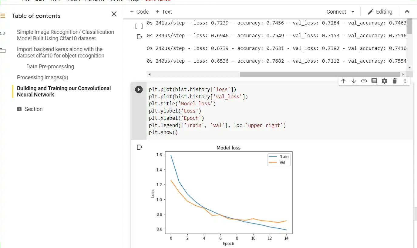
Before using this model to make some predictions, let’s plot some learning curves that would help us understand how well our model trained. this step should help us understand overfitting, underfitting, unsteady training and so on. This can help us to decide steps to take that can help improve the model.

Plot showing Model Loss during Training

…..

Plot showing Model Accuracy during Training

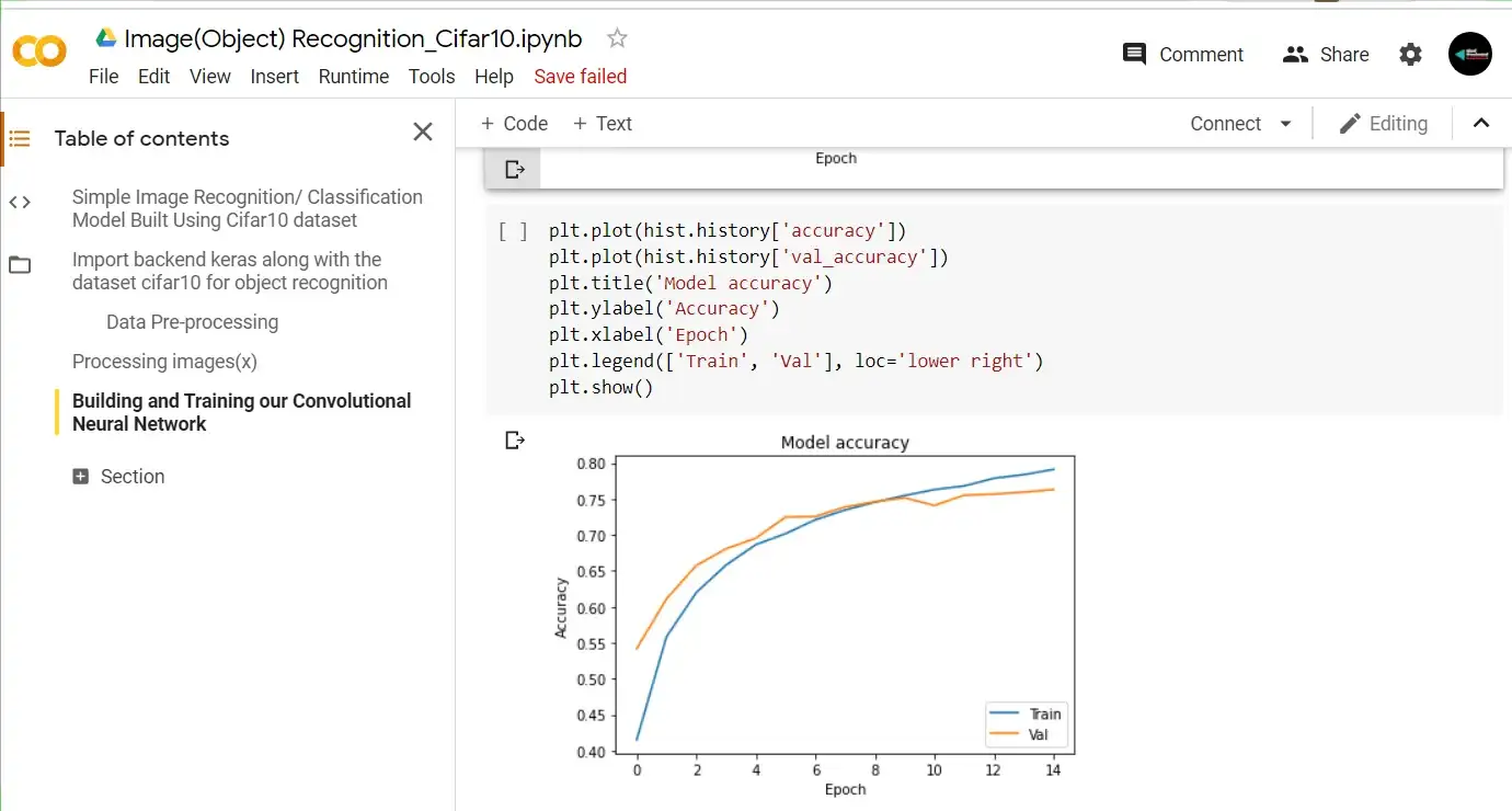
From the above plots we see that, we had a steady training without overfitting our model. Now for the last step, we want to evaluate our model using the test set and also make predictions using entirely new images. You can do this by getting images that fall into any one of the classes as we have in our dataset. The code below would enable you to choose multiple files from your storage for prediction.

model.evaluate(x_test, y_test_one_hot)[1]
model.save('chel_cifar10_model_OR.h5')

import numpy as np
from skimage import data, color, feature, transform
from skimage.transform import resize
from google.colab import files
from keras.preprocessing import image

uploaded = files.upload()
for fn in uploaded.keys():

path = '/content/' + fn
img = image.load_img(path, target_size=(32, 32))
x = image.img_to_array(img)
x = np.expand_dims(x, axis=0)

#images = np.vstack([x])
probabilities = model.predict(images, batch_size=10)
print(probabilities[0])

number_to_class = ['airplane', 'automobile', 'bird', 'cat', 'deer', 'dog', 'frog', 'horse', 'ship', 'truck']
index = np.argsort(probabilities[0,:])
print("Most likely class:", number_to_class[index[9]], "-- Probability:", probabilities[0,index[9]])
print("Second most likely class:", number_to_class[index[8]], "-- Probability:", probabilities[0,index[8]])
print("Third most likely class:", number_to_class[index[7]], "-- Probability:", probabilities[0,index[7]])
print("Fourth most likely class:", number_to_class[index[6]], "-- Probability:", probabilities[0,index[6]])
print("Fifth most likely class:", number_to_class[index[5]], "-- Probability:", probabilities[0,index[5]])

The above code evaluates our model using test set, saves the trained model in a .h5 format and also we are able to upload files for prediction by the files library from keras. Then we converted the output numbers into words_class as it’s easier to understand that way. The last bit of code enables us to do that.

After training the model and evaluating on the test set (x_test), I got an accuracy of 75%. This means that, our classifier would classify correctly only 75% of new unseen images we feed it.

Test out different images to see how well the model you built classifies them.

In the part 2 of this article, let’s look at how to Improve significantly our built model’s accuracy by Introducing some new concepts that would prevent over-fitting and slow down convergence. Next Article: Improving your Tensorflow Model with Dropouts and Batch Normalization