Introduction to Linear Regression - Creating a Simple Learning Predictor
May 31, 2020

So now that you know a little bit about Machine Learning. It becomes natural for you to understand how you can use it to build models that are capable of making decisions at minimal level. The way we achieve this is the use of Machine Learning Algorithms that were developed several years back by experts in the field.
The way these algoritm are capable of learning from real-world data to be able to make predictions is mostly because the mathematical computations on which they are built support or are proven to learn or map data to specific labels through probability and with experience.
In this article, you would be introduced to one of the simplest and popular ML Algorithm called Linear Regression. It is recommended that you read our tutorial on Vectorization with Matlab if you haven’t already as we would be using vectorization to implement our LR model for faster and easier bug debugging.
Linear Regression is a Machine Learning algorithm that is used for predictions of “continuous /non-classified data”. To better understand it, let’s use a very popular example. Say, you want to predict the prices of particular houses,height of students in a class, weight and so on. This examples define continuous data, that is, they stand alone and are not grouped into classes. This is in contrast to a second learning algorithm called Logistic Regression which we would be looking at in the next post. Before we proceed to the implementation of Linear Regression, i want to give a general idea or intuition about what an ML model is trying to achieve and how it works.
I learnt Linear Regression from the Stanford University Machine Learning course on Coursera taught by Professor Andrew Ng. I feel like i could not have gotten a better understanding if i had learnt it elsewhere, Andrew always wanted to give the students an intuition about any new algorithm we were taking on and i loved it. It made me understand exactly how that algo was different from the previous one even before we started learning the maths behind it. I should say, that’s one of the best course or teaching i have ever received. Now i have this understanding of the different algoritms that even if i were to forget the correct code to implement them i still have a very good grasp of what they are doing and i think that’s very important.
Now i would give you guys that intuition at the start of every algo you would be learning.
You have some datasets in continuous values(because we are doing LinearRegrssion) and you want to go about training a model to the point that it achieves a preferred level of accuracy that you consider good enough for the use you want. Yh yh, we want a model that can do that for us but how does it come to achieve this?. In Machine Learning we have two main types of model learning; supervised and unsupervised. To get more insights on them, read our full article on Machine Learning. In Linear Regression we are carrying out the supervised part of learning, think of it as supervised beacuse we are providing some labels or correct values that we want our model to learn from. It goes exactly like this: we have a data set we a number of examples, each of this examples has two values in a row (x and y). The x denotes the value that is fed into the model and y denoting the output of the model. These x’s and y’s are both fed to the model during the training step/phase, therefore the name supervised. When we begin to do the math of it, i would explain i details what these terms mean and you should hopefully understand it better.
We have some specific steps of training that we would take iteratively or repeatedly, the main purpose of this is to reduce the errors generated at each trainng step or loop. Its almost as easy as that. Now we come to the algoritms involoved that helps us achieve that.
THE THREE MAIN CODE IMPLEMENTATION WHEN TRAINING A LINEAR REGRESSION ALGORITHM:
- Prediction function
- Cost Function
- Gradient Descent
Let’s look at each of them closely. We know we want an accurate “predictor”, and for that to be, three things has to happen: Our model could start by randomly guessing or well thinking at least it’s guessing correctly but the model would definitely be wrong because initially it hasn’t mapped a function to the data, now we use the cost function to calculate the errors gotten on all our training examples of that step in the loop,that is. the errors when our predictor tried to guess what the output y’s of each x’s were. Finally, the Gradient Descent algo tries to fit our model better by reducing the amount of those errors until it converges to a point that the errors are minimal or can’t be reduced further. Now i would define all the most of the terms used in Linear Regression so you can understand better what each is doing.
-
Dataset: Dataset is a collection of data, usually data fron real world affairs that can be used to train a model. It can be in either structured or unstructured form. The stuctured type of data can be divided into supervised or unsupervised datasets. Datasets sizes ranges from hundreds of trainig examples to as much as millions. Data is usually the first step of model training referred informally as “collecting data”.
-
Algorithm: A set of mathematical or statistical calculations that is used to compute for numbers, they are proven to give us our answers if implemented in the correct order. Algorithms are found in different fields of study, each constucted to be abstracted will also supporting some higher-level logic for the purpose it’s used.
-
Training Examples: Usually found in the dataset, training examples in Linear Regression consists of some x’s and y’s which we want our model to learn from considering they are the correct form of matching or mapping that we want. Think of the input x as any subject that can be used to ‘determine’ an effect or some other number. And y being that number that was the result of exactly what x is. So let’s just say they are dependable of themselves.They are denoted by m
-
Cost Function: A function in Machine Learning that is always given the task of finding errors after one iteration of learning or after our “predictor” as tried to guess the output of all x’s. Different ML algorithms would come with cost functions that are constructed for exactly how they are used or what concept they support, that in most cases would not work for a different Ml Algorithm. We would call the output y the model is trying to predict y hat. Consequently, this cost-function is the difference between yhat and y matched be some parameter theta. They are denoted by capital J
-
Parameters: In Linear Regression, we are trying to predict our y’s given x’s. How we achieve this is that we use parameters called theta to map the function for us. These theta are practically the ones that gives us our errors and by changing them, we can get smaller errors and so on. They are what the model is built upon. In Linear Regression, parameters theta multiplied by our input data x gives us our prediction of ouput y. So you can see how important they are, we use gradient descent to change or reduce the errors calculated by cost function and by changing those errors our parameters theta are defining the predictions a bit more correctly, that is, they are getting better.
-
Gradient Descent: Gradient Deascent is a powerful algorithm that is used in Linear Regression to update theta to a value that gives less errors. It is an iterative function that keeps updating theta in every cycle of the loop until theta converges or gets to the point that it’s reduction if any becomes insignificant.
So now you know the three main steps involved in Linear Regression and hopefully the basic definitions of those terms gave you a better idea of how we train a Predictor or model. Now we can go ahead to implement all these in code. For this tutorial, I would get a dataset of one feature X and output Y from Open ML,a platform where ML engineers and data scientists can collaborate on projects or share datasets. I will be implementing and testing the code written here on MATLAB, a platform for carrying out mathematical computations and linear algebra. It comes with a free-trial, but to use for an extended period of time, a fee has to be paid. If you want to follow along, you can either use MATLAB or OCTAVE. To set up octave, read our article on how to set up octave on windows.
So I downloaded a dataset from open ML to my PC, I can then login to my MATLAB acct, upload the data, and start building a Linear Regression predictor. Let’s Begin
AIM OF PREDICTOR
In this tutorial we would be building a simple model that would use a number of input features x to predict the ‘price’ a building will sell for.
DATASET
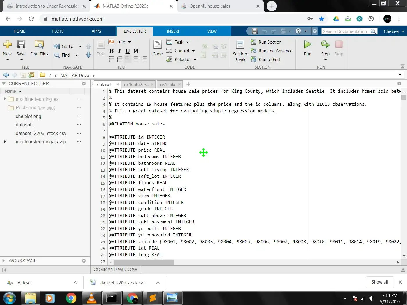
This dataset contains house sale prices for King County, which includes Seattle. It includes homes sold between May 2014 and May 2015.

It contains 19 house features plus the price and the id columns, along with 21613 observations. It's a great dataset for evaluating simple regression models.
You can download this dataset from OpenML here. As stated it is a multi-varaint dataset or simply, it has multiple features in total 19, and 21613 training examples. For this tutorial, we would be using 3 features and 100 training examples.To implement for a uni-variant model, you can follow the whole process but instead load just one feature into the x variable. You would learn about it all soon.
FEATURES
The 3 features we would be giving our variable x are number of bedrooms, sqft of living area and year built. There a a lot more features but the reason i chose those 3 is because they seem like the factors that play the largest role of influence on the price a customer would like to pay for a house. Also including similar features like sqft of basement , sqft of upperlevels and so on would end up making the features redundant (repetitive or duplicating). Take a look at the full features in our dataset.

To set off,we would be using the list as a guide to know the order of the steps it takes to build our model.You can always refer back to this, as a reminder of what steps you should be implementing at what time.
- Feature Normalization
- Plot the Data
- Compute for the Cost Function
- Gradient Descent
There is a step included that we have not yet covered, let’s do that now.
Feature Normalization is a way to neutralize the wide range of values we might have in our dataset. It simply reduces how far apart how data is in their real values in numbers. For example, in our house_sales dataset we can observe that the difference between the year_built and no_of_bedrooms features is so wide apart and can cause irregularities for our model to learn accurately in lesser time. The way to combat this is simply to normalize our data. In Machine Learning this is referred to as “Feature Normalization”.
Plotting data is a good way to understand our data, it can be done at different steps when implementing ML algorithm, apart from the purpose of visualization, it also helps us for debugging just by looking at the curves and shapes our data takes.You would learn more about this in future lessons. To plot the data onto a graph, we use a set of built-in functions from MATLAB (same applies in Octave). Whenever i use some new built-in function in our code I would give a brief explanation of what it does, for this reason, anyline starting with a “%” signifies an explanation of the code on the next line. The “%” sign is the official way used to write comments in Matlab.
Now let’s begin with the first step on the list, which is loading our data into MATLAB Environment normalizing our features so when plotting we can have a better idea of our data.
Load the Data into Environment
% Load Data
data = load('dataset_');
% Load into X , row 1-100 and columns 4 , 6 & 15
X = data(1:100, [4,6,15])
% Load into y, row 1-100 column 3 (price)
y = data(1:100, 3)
% Denotes the number of training examples , length (100)
m = length(y)
% Call the pre-defined func "featureNormalization"
% It takes one value X and computes three values, (X_normalized, mean of X , range of X)
[X, mu, sigma] = featureNormalize(X)
% Plot the dataset using the normalized X
plot(X,y,'r*')
% Print out first 10 examples from the dataset
fprintf(' x = [%.0f %.0f %.0f], y = %.0f \n', [X(1:10,:) y(1:10,:)]');
FeatureNormalization.m
Xfunction [X_norm, mu, sigma] = featureNormalize(X)
%   FEATURENORMALIZE(X) returns a normalized version of X where the mean value of each feature is 0 and the standard deviation is 1.
% This is often a good preprocessing step to do when working with learning algorithms.

% You need to set these values correctly
X_norm = X;
mu = zeros(1, size(X, 2));
sigma = zeros(1, size(X, 2));

% First, for each feature dimension, compute the mean of the
% feature and subtract it from the dataset,storing the mean value in mu.
% Next compute the standard deviation of each feature and divide each feature by it's standard deviation, storing the standard deviation in sigma.
% Note that X is a matrix where each column is a feature and each row is an example.
% You need to perform the normalization separately for each feature.
% Hint: You might find the 'mean' and 'std' functions useful.
mu = mean(X);
sigma = std(X);
X_norm = (X - mu)./sigma;


end
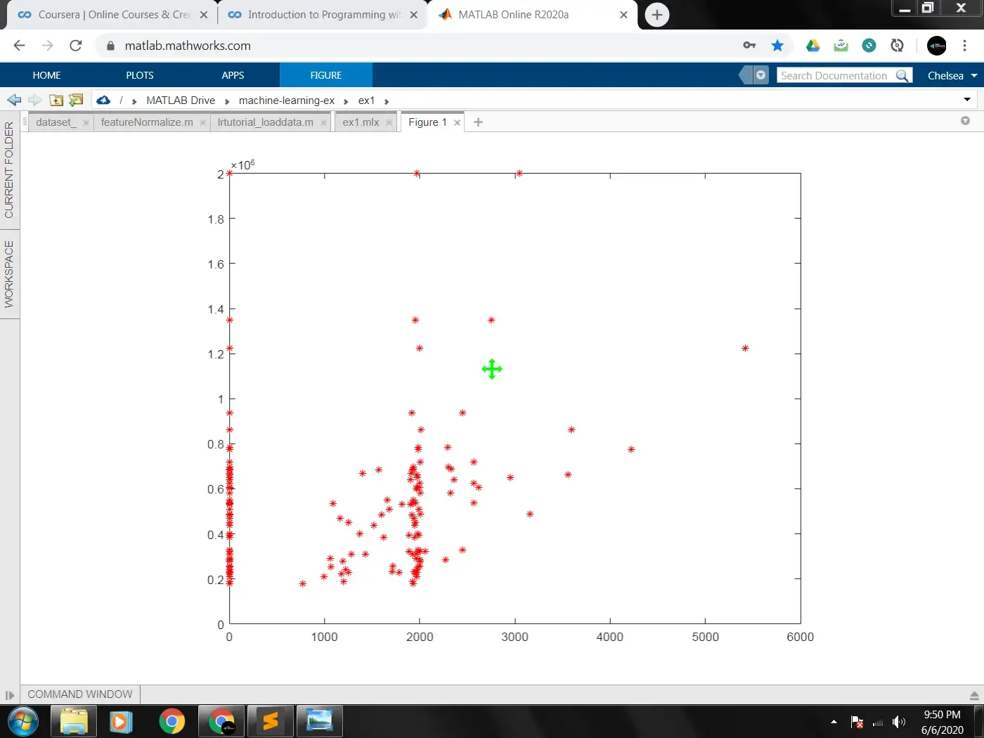
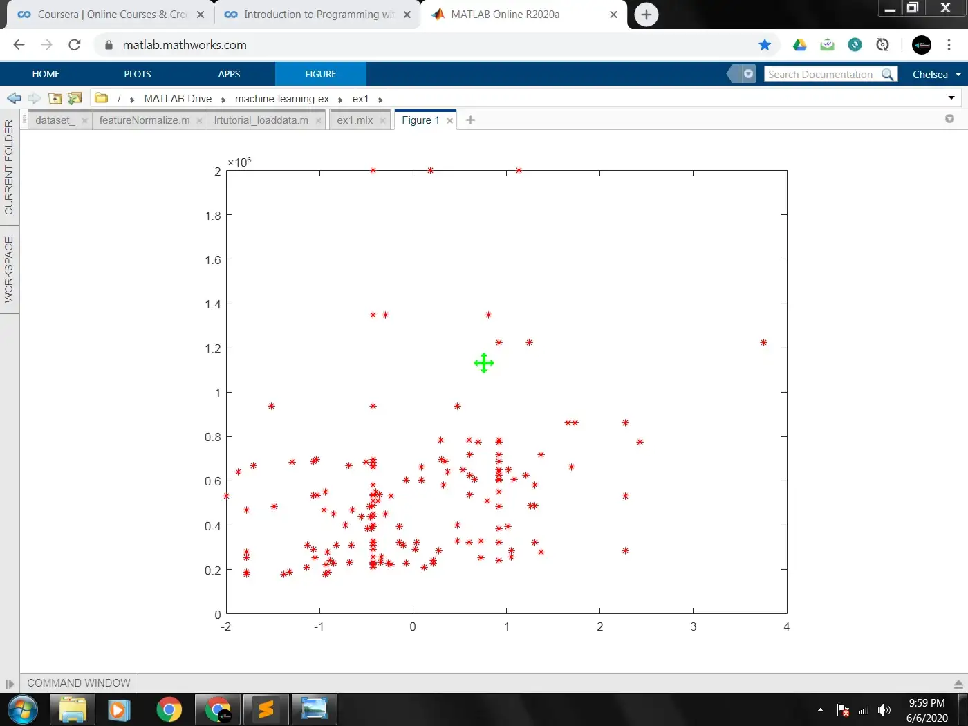
To make you understand better what feature normalization does, Below are two images showing the plot when the features of X are normalized against when they are not.
RAW DATASET(UN-NORMALIZED)

FEATURE NORMALIZED

As you can see,, in the un-normalized plot of our data, we have some of our points directly on the y axis. This is because the range between our dataset is to wide causing some of the smaller values of X to take their places as close as possible to the line. Normalizing our data sets them all in the same range.
Now we have completed the first step, X an y now holds the values we want them to. These values are what we use to train the model for future house_price predictions. The next step on the list is Compute the cost func. Cost function tries to calculate the value of ‘theta’ that gives the lowest cost/error when it predicts the values that y’s should be. Let’s write the code for it
Compute Cost Function
% Add intercept(bias) term to X
X = [ones(m, 1) X];
function J = computeCost(X, y, theta)
% J = computeCost(X, y, theta) computes the cost of using theta as the parameter for linear regression to fit the data points in X and y
% Initialize some useful values
m = length(y); % number of training examples
% You need to return the following variables correctly
J = 0;
% Compute the cost of a particular choice of theta
J = (1/(2*m))*(sum(((X*theta)-y).^2));

end
So for the above code, we can see that J is given the value of the cost. The formula above is what is used to compute for cost func in Linear regression. We are constantly multipliying parameters theta and X and subtracting it from our prices y, this helps us to finally calculate the overall cost which we can use in GradientDescent alogrithm to correct. The alogrithm used to compute the costFunction is called “squared error term” , as we are squaring the error of ((X * theta)-y)
Now for the Gradient Descent Algorithm. Here, in simple terms we are using the error term computed to learn a better value for our parameters theta. To make you understand better, in gradient descent we are trying to minimize the cost J, for us to do that we need to find the best fit to the data that gives the lowest error i.e, the distance from the points our x’s are located on our data plot is small. Gradient Descent minimizes our cost function on every iteration(loop) of the algorithm, it does this by finding the derivative of J with respect to our parameters and updates J based on this. Finding the derivative simply means, how much does theta affect the cost and minimizing it to attain a global minimum(a point where theta does not change significantly anymore). Now let’s look at the code for Gradient Descent.
Learning Rate Alpha is an hyperparameter in Machine Learning that controls the amount of step taken by gradient descent takes in one iteration of learning parameters theta
Compute Gradient Descent
function [theta, J_history] = gradientDescentMulti(X, y, theta, alpha, num_iters)
%theta = gradientDescentMulti(x, y, theta, alpha, num_iters) updates theta by taking num_iters gradient steps with learning rate alpha
m = length(y);
% the index of the number of iterations
J_history = zeros(num_iters, 1);
%looping over the total num of iterations
for iter = 1:num_iters
% calculating the error
error = (X * theta) - y;
% updating theta
theta = theta - ((alpha/m) * X'*error);
end
From the above code, after gradient descent completes , we should have 3 Theta values, becasue we used only three features of X from our dataset. Having more features would mean more theta parameters since theta is the learned parameter that enables us to make predictions on new data having three features in our case.
That’s all for Linear Regression, we now have our trained model capable of making predictions. In the below and final code we now make a prediction with new unseen data of X of what the price of a house(y) should be or a very close estimate.
Predict on New Data
% Estimate the price of a 1650 sq-ft, 3 br house
X = [1650,3];
% Feature Normalize the data
featureNormalize(X);
X = ones(:1,X)
% Final prediction price
price = [X].* theta; % Enter your price formula here
That brings us to the end of this tutorial, we implemented Linear Regression, perhaps the simplest Machine Leraning Algorithm there is, and i would recommend going through it a few times to you know, improve your intuition on how the code works and also familarize yourself with the code involved. For the code, it’s always possible to copy it down somewhere, refer to it a few times because at first, it wouldn’t stick straightaway but after using it a few times it becomes natural to your senses, I know that because I’ve been in the same sitution. During my first few weeks learning Machine Learning by Andrew, it was overwhelming for me, i got a good understanding of the concepts, intuition but the code was quite strange and hard for me to grasp, but honestly now my eyes passes through the details whenever I’m working with Linear Regression Algo, and I know that would be the same for you.
In the next article , I would give an Introduction to Logistic Regression and you would see how to build a classification model using the Algorithm. Thanks for reading , I hope i’ve been able to uncover and actually simplify Linear Regression Algorithm for you, and with these steps you can go ahead learning the other types we have and you know implementing the ideas and code we looked at. As always, there are nimble steps to take towards finding the right platform, tools, or communities. I would love to read any comments you have about this article or other areas of ML, please feel free to leave a comment below.